Load libraries.
library(eDASH)
#> Registered S3 method overwritten by 'quantmod':
#>   method            from
#>   as.zoo.data.frame zoo
#> Warning: replacing previous import 'dplyr::summarise' by 'plyr::summarise' when
#> loading 'eDASH'
library(ggplot2)
Preliminary inspection of the dataset.
df <- eDASH::data
head(df)
#> Date_Time Weekday Month ToU Total_Power Chiller Hglobal Text
#> 1 2015-04-01 00:00:00 Mer Apr F23 184.8 2.8 0.2 18.5
#> 2 2015-04-01 00:15:00 Mer Apr F23 162.4 2.8 0.1 18.4
#> 3 2015-04-01 00:30:00 Mer Apr F23 186.8 2.8 0.2 18.3
#> 4 2015-04-01 00:45:00 Mer Apr F23 164.8 2.8 0.2 18.1
#> 5 2015-04-01 01:00:00 Mer Apr F23 179.6 2.8 0.3 18.1
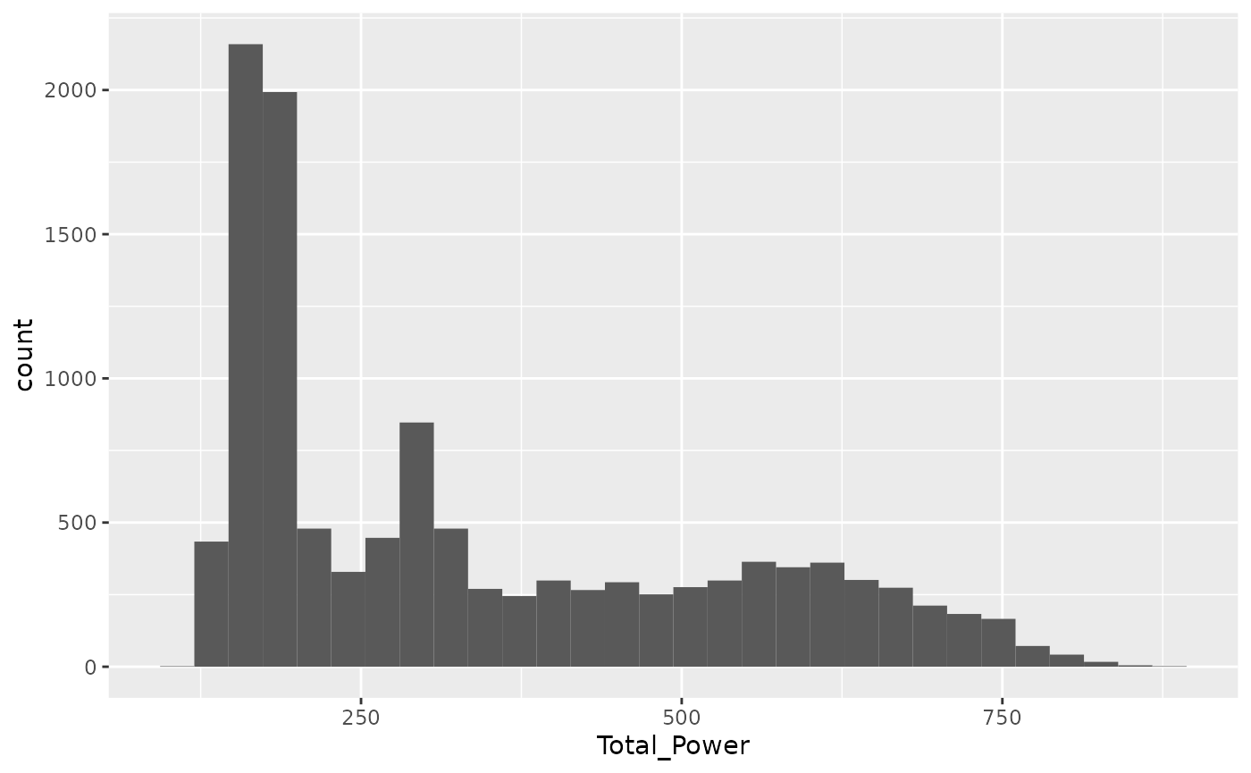
#> 6 2015-04-01 01:15:00 Mer Apr F23 175.2 2.8 0.3 17.9Plot distributions
ggplot(df)+
  geom_histogram(aes(x = Total_Power))
#> `stat_bin()` using `bins = 30`. Pick better value with `binwidth`.